Fundamental building blocks of effective computation | Subscribe


A data structure is a way of organizing and storing data in a computer so that it can be efficiently accessed and manipulated. It provides a systematic way of organizing and managing data to facilitate efficient operations like insertion, deletion, and retrieval of data items.
For all new updates: Subscribe
Data structures are the fundamental building blocks of effective computation in the field of computer science. They offer the structure for managing, processing, and storing data to enable smooth operations. However, selecting the right data structure by itself is insufficient to ensure top performance. Time complexity is a notion that is used to quantify the effectiveness of algorithms and how they interact with data structures. In this blog, we’ll go into the world of time complexity and discuss the significance of data structures, highlighting how crucial it is for creating effective algorithms.
For all new updates: Subscribe
What is Data Structure(s)?
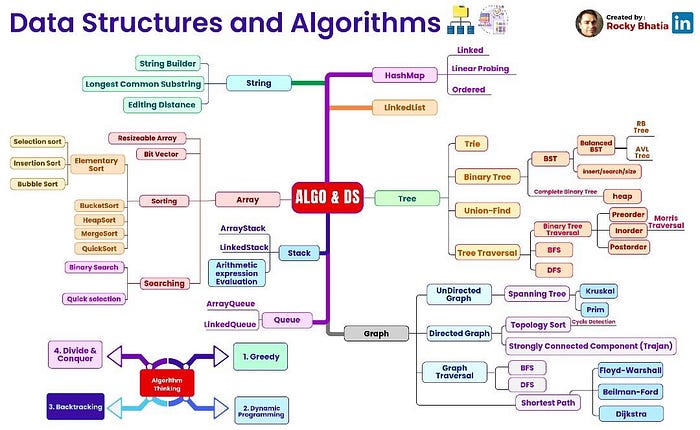
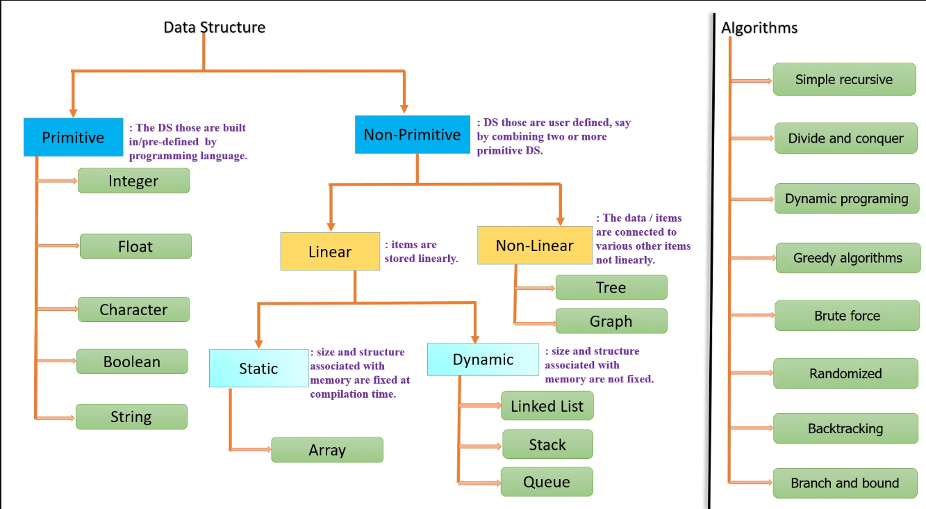
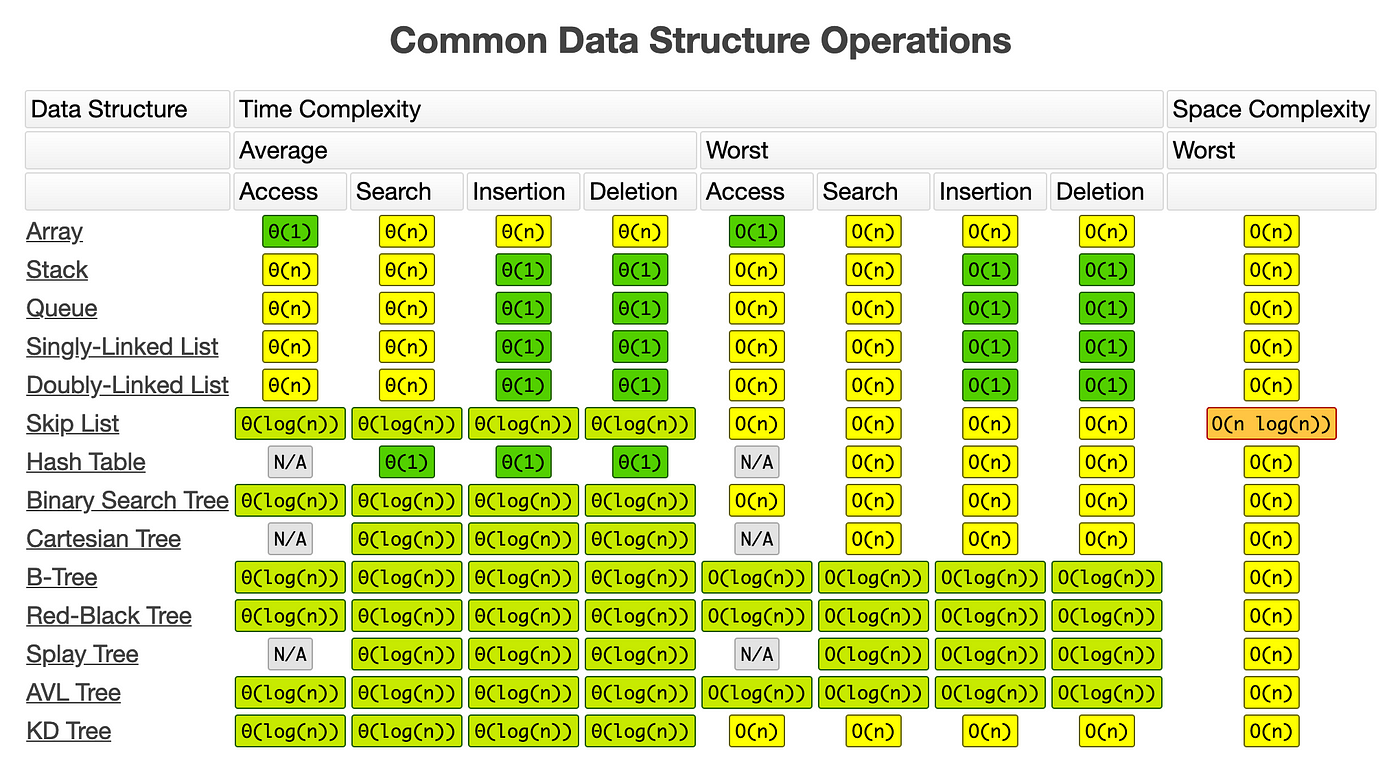
Data structures are specialised formats for classifying and archiving data to make data retrieval and manipulation easier and more effective. They are created to fulfil certain needs, maximise memory usage, and improve algorithm speed. Arrays, linked lists, stacks, queues, trees, graphs, and hash tables are examples of frequently used data structures.

Each data structure has distinct qualities that define which activities it is best suited for. For instance, while arrays provide constant-time access to their elements, their size flexibility is constrained. Linked lists, on the other hand, provide dynamic memory allocation but have slower access times to their elements. Understanding the trade-offs and intricacies of different data structures allows us to select the best one for a specific task, maximizing productivity and resource use.
For all new updates: Subscribe
Time Complexity: Measuring Algorithm Efficiency
Algorithms give data structures life, while data structures provide the framework. Algorithms are detailed processes created to address particular computational issues. The length of an algorithm’s runtime about the size of the input is a measure of an algorithm’s time complexity. It enables us to assess, contrast, and forecast the effectiveness of various algorithms given various input sizes.
There are again 3 different types of complexity that come to the picture such as:
Big O (Big O): A complexity that is going to be less than or equal to the worst time a program can take.
Big Ω (Omega): It is a complexity that is going to be at least more than the best case.
Big θ (Theta): It is a complexity that is within the bound of the worst and the best case.
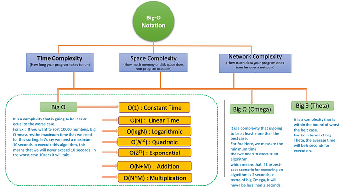
Big O notation, which depicts the upper bound of an algorithm’s runtime as a function of the input size, is frequently used to explain time complexity. For instance, an algorithm with an O(1) time complexity runs in constant time, regardless of the quantity of the input. An algorithm with O(n) time complexity, on the other hand, denotes that the runtime increases linearly with the size of the input.
The best algorithm to do a task can be chosen by understanding temporal complexity. It helps us to consider the predicted input size and required performance levels when choosing data structure options and algorithm designs. We can find possible bottlenecks, improve algorithms, and ultimately arrive at quicker and more scalable solutions by analysing temporal complexity.
Some common Time Complexities and their characteristics
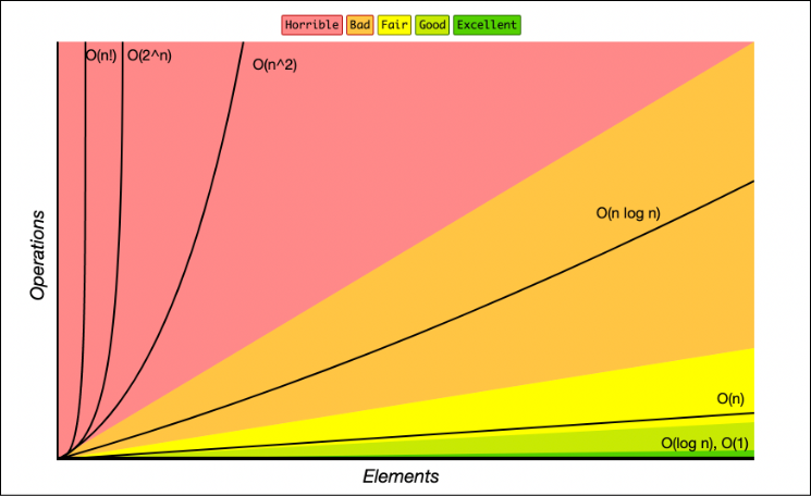
O(1) — Constant Time Complexity
- Regardless of the size of the input, an algorithm with constant time complexity runs for a fixed period. It is regarded as the most effective time complexity. This includes operations like retrieving an element from an array or carrying out a simple mathematical operation.
Example: Retrieving the first element from an array, regardless of the array size, takes constant time.
O(log n) — Logarithmic Time Complexity
- We can call it as Big O of one or O of one, which is a constant time complexity, where for any given input, the execution time will not change. It will remain constant regardless the increase or decrease of input data set N. Eg.: Accessing a specific index within the array always takes an O(1) time complexity.
- This type of algorithm has a runtime that increases logarithmically as the amount of the input. It frequently happens in algorithms, such as binary search, that break up the input into smaller pieces at each stage. Although more slowly than with linear time complexity, runtime grows as input size does.
Example: Binary search in a sorted array divides the search space in half at each step, resulting in logarithmic time complexity.
O(n) — Linear Time Complexity
- Big O of N or O of N is a linear time complexity where time complexity will grow in a direct proportion to the size of the input data.
Ex.: Traversing through all the elements in a given array.
- A linear time complexity algorithm has a runtime that increases linearly with input size. In proportion to the size of the input, the runtime grows as well. This category frequently includes algorithms that run iteratively across an array’s elements or carry out a single operation on each input member.
Example: Computing the sum of all elements in an array requires visiting each element once, resulting in linear time complexity.
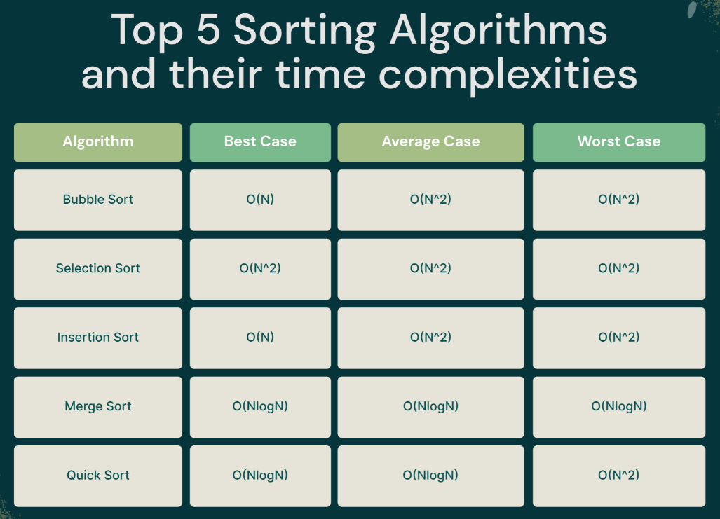
O(n log n) — Linearithmic Time Complexity
- Big O of log N or Log O of N is a logarthimic time complexity, where the complexity proportional to the logarithmic of the input. Ex.: Finding an element in a sorted array.
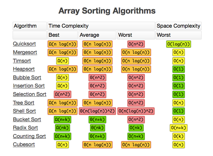
- An algorithm with a runtime that grows linearly but additionally depends on the logarithm of the input size is said to have a linearithmic time complexity. It can be found frequently in sorting algorithms like quicksort and merge sort.
Example: Merge sort divides the input into smaller parts recursively and then merges them back together, resulting in a linearithmic time complexity.
O(n²) — Quadratic Time Complexity
- The time complexity of an algorithm is refered as Big O of N² or O of N² , whose performance is directly proportional to the square size of input dataset(N).
Ex.: Traversing through every index in an array twice.
- The runtime of an algorithm with quadratic time complexity increases exponentially as the input size increases. When each input element must be compared to or processed concerning each other element, it happens. Nested loop algorithms frequently have quadratic temporal complexity.
Example: Bubble sort, which repeatedly compares and swaps adjacent elements, has a quadratic time complexity.
O(2^n):
Big O of 2 to the power of N or exponential time complexity is an algorithm whose growth doubles with each addition to the input data set. Eg. Double recursion in a fibonaci series.
O(N + M):
If an algorithm is in the form of “ do this first and when you are all done, do that” then you add the runtime. For ex. Loop through all the element in array A and then loop through the element in array B.
O(N * M):
If an algorithm is in the form of “ do this for each time you do that” then you multiply the runtimes. For example a nested loop where for each iteration of the first loop the second loop iterates till M times.
Rules of measuring Big O time complexity of an program:

Data structures and their Real-life applications
↪ Arrays
- Real-life example: Shopping lists.
- Arrays are one of the simplest data structures and consist of a fixed-size sequence of elements of the same data type. They provide fast access to elements by their index but have a fixed size and can be inefficient for inserting or deleting elements.
- Why — A shopping list can be represented as an array where each item corresponds to an element in the array. Arrays provide efficient random access to elements, making them suitable for storing and retrieving a list of items.
↪ Linked Lists
- Real-life example: Train cars connected.
- Linked lists are dynamic data structures that consist of nodes linked together by pointers. Each node contains a data element and a pointer to the next node. Linked lists allow efficient insertion and deletion at any position but have slower access time compared to arrays.
- Why — Linked lists consist of nodes that are linked together using pointers. Similar to train cars being connected to form a train, linked lists maintain a sequence of elements where each node points to the next node. Linked lists provide efficient insertion and deletion at any position in the list.
↪ Stacks
- Real-life example: Undo/Redo functionality in text editors.
- Stacks are abstract data types that represent collections of elements. Stacks follow the LIFO principle, where elements are inserted and removed from the same end called the top.
- Why — A stack follows the Last-In-First-Out (LIFO) principle. Just like the undo/redo feature in text editors, where the most recent action is undone or redone first, a stack allows adding and removing elements from the top only.
↪ Queues
- Real-life example: Supermarket checkout lines.
- Queues follow the FIFO principle, where elements are inserted at one end called the rear and removed from the other end called the front.
- Why — Queues operate on the First-In-First-Out (FIFO) principle. Similar to customers lining up at a supermarket checkout, a queue data structure allows adding elements at the rear and removing them from the front, ensuring that the first element added is the first one to be processed.
For all new updates: Subscribe
↪ Trees
- Real-life example: Organisation hierarchy.
- Trees are hierarchical data structures composed of nodes connected by edges. They have a root node and each node can have child nodes. Trees are commonly used for representing hierarchical relationships and can be binary trees (each node has at most two children) or n-ary trees (each node has any number of children).
- Why — Trees are hierarchical data structures. A common real-life example is an organisation hierarchy, where each employee represents a node, and the relationships between employees form a tree-like structure. Trees provide efficient searching, sorting, and hierarchical representation of data.
↪ Graphs
- Real-life example: Social networks.
- Graphs are a collection of nodes connected by edges, where each edge can have a direction (directed graph) or not (undirected graph). Graphs are used to represent complex relationships and can have various algorithms and data structures associated with them, such as adjacency matrices or adjacency lists.
- Why — Graphs consist of nodes (vertices) connected by edges. Social networks, such as Facebook or LinkedIn, can be represented as graphs, where individuals are nodes, and connections between individuals are edges. Graphs are used to model relationships and connections in various real-life scenarios.
For all new updates: Subscribe
↪ Hash Tables
- Real-life example: Dictionary.
- Hash tables are data structures that use a technique called hashing to store and retrieve elements based on their keys. They provide fast insertion, deletion, and retrieval operations on average, making them suitable for implementing dictionaries and databases.
- Why — Hash tables are data structures that use key-value pairs. A dictionary can be implemented using a hash table, where words serve as keys, and their corresponding meanings serve as values. Hash tables provide efficient lookup and insertion based on the key.